pBRIT candiate gene prioritization

Documentation: Introduction

pBRIT prioritizes candidate disease genes in a three-staged methodology. The main steps, and principles are discussed below.

Stage 1 : Feature Mining

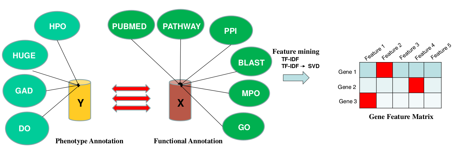
pBRIT integrates 10 annotation sources, categorized as either functional or phenotypic, as illustrated in the figure above. Under the functional class, we included Pubmed Abstracts, Pathways, Protein-Protein Interactions, Protein sequence similarities (BLAST), Mouse Phenotype Ontologies (MPO) and Gene Ontology. Phenotype annotations were included from Human Phenotype Ontology (HPO), Genetic association database (GAD) and Disease Ontology (DO).

More specifically, pathway information included data from Biocarta, EHMN, HumanCyc, INOH, KEGG, NetPath, PharmGKB, PID, Reactome, Signalink, SMPDB and WikiPathways. Similarly, PPI information was gathered from PhosphoPOINT, PDZBase, NetPath, PINdb, BIND, CORUM, Biogrid, InnateDB, MIPS-MPPI, Spike, Manual upload, MatrixDB, DIP, IntAct, MINT, PDB and HPRD.

All the annotation matrices except BLAST are represented as sparse binary matrices. Next, TF-IDF, an unsupervised approach towards feature mining, is applied to assigning statistical weights to individual features:

$$\textbf{TF}(f,g) = 1+\textbf{log}(\textbf{tf}_{feature, gene}) \\ \textbf{IDF}(f,G) = \textbf{log}(\frac{|G|}{1+|\{g\epsilon G : f\epsilon g\}|}) \\ \textbf{W}(f,G) = \textbf{TF}\times\textbf{IDF} $$

The term frequency (tf) is equal to one due to the binary data format. IDF(f,G), or inverse document frequency, denotes the inverse frequency of a particular feature (f) across all genes (G). Hence, it describes the specificity of a feature. W(f, g) gives the statistical weight of feature (f) for a given gene (g). Using TF-IDF, specific features get higher weights, contributing more to the final similarity score used in ranking.

Finally, we applied Singular Value Decomposition (SVD) on TF-IDF weighted annotation matrices, to model co-occurrences and latent semantic dependencies between the features . This is denoted as TF-IDF→SVD or TF-IDF transformed using SVD. During SVD, each annotation matrix was decomposed in k singular values and then projected in those directions. The optimal choice of k corresponds to a maximal preservation of variance in the data. In our case, k was set to 200 for all annotation sources. Mathematically, this can be expressed as:

$$A_{m\times n} \approx U_{m\times k}D_{k\times k}V_{k\times n} \\ \tilde{A}_{m\times k} \approx A_{m\times n}V_{k \times n}^T$$

Stage 2 : Intermediate Data Intregration

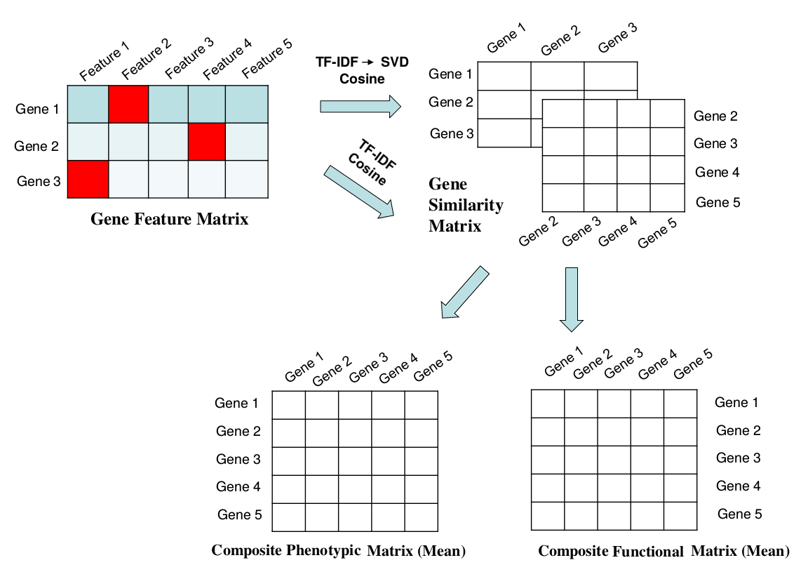
We can then calculate gene-by-gene similarity for each annotation source by taking the Cosine of the respective TF-IDF weighted annotation matrices. Composite matrices are constructed by taking inter-matrix means over all functional or phenotypic annotation category:

$$X_{composite} = \frac{\sum_{f}^F { X_{f}}}{F} \\ Y_{composite} = \dfrac{\sum_{p}^P { Y_{p}}}{P}$$

These composite matrices are the final similarity matrices incorporated into the regression model.

Stage 3 : Construction of the regression model.

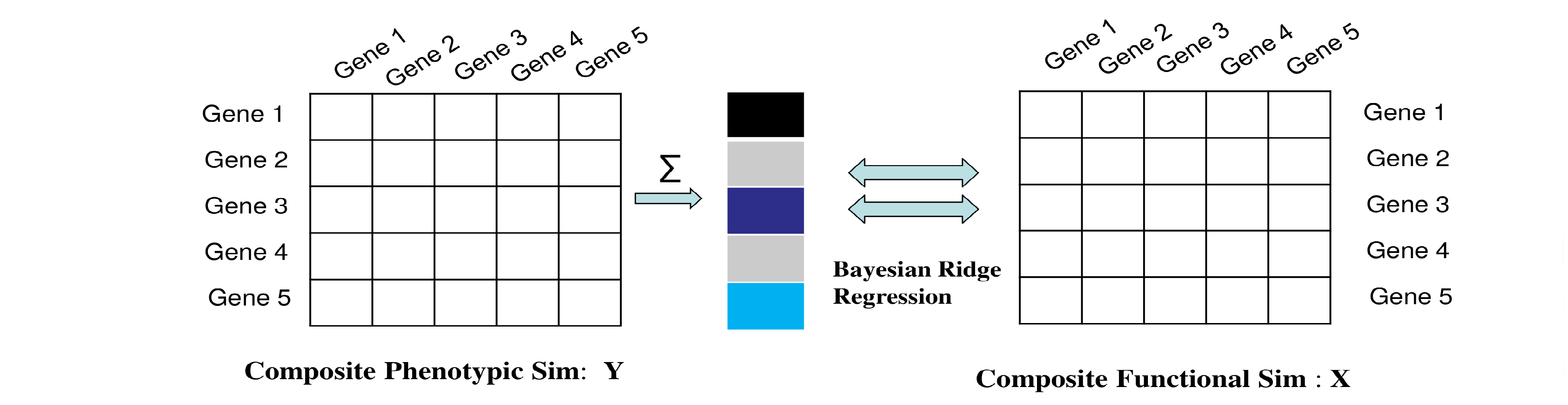
For a given set of training genes, gene-by-gene similarity matrix are retrieved for both functional and phenotypic annotations sources. Next, phenotypic similarities are summed over all training genes (columns), to yield a single value per gene under consideration (rows).

We can then define the regression model as:

$$Y_{(n+m)\times 1} = \beta X_{(n+m)\times n} + \epsilon $$

Where the error term $\epsilon \thicksim N(0|\sigma^{2}_{\epsilon})$. The unknowns, the regression coefficient $\beta$, its corresponding variance $\sigma_{\beta}^2$ and the residual variance $\sigma_{\varepsilon}^2$ can be estimated uniquely. In order to overcome over-fitting and multi-collinearity due to relatedness of the training genes, we regularize the estimates by adding a parameter $\tilde\lambda$ which is given by the ratio of $\sigma_{\varepsilon}^2 / \sigma_{\beta}^2$. As the $\sigma_{\beta}^2$ increases to larger values the solution to find optimal $\hat\beta $ approximates ordinary least squares estimates. Requirements for the optimal choice of $\hat\beta$ are given by:

$$\hat{\beta} = \underset{\beta}{\mathrm{argmin}} \left\{ \sum_{i=1}^{n+m}(y_i - x_i^T \beta)^2 + \tilde{\lambda} \sum_{j=1}^{n} {\beta_j}^2\right\} \\ E(\beta\mid y)= \hat{\beta} = \left[ \textbf{X}^T X + \tilde{\lambda} I\right]^{-1} X^Ty$$

Full details on the bayesian model, the chosen priors (NIG) and the joint posterior distribution can be found in the manuscript. Since posterior distribution of unknowns in the model does not have closed form, we applied a Gibbs sampler to perform parameter estimation.

Stage 4 : Gene Prioritization.

Once the parameters of the regression model are estimated, the corresponding phenotype concordance is calculated for each test gene. By ranking these scores, the final prioritization is performed. Mathematically, the phenotypic concordance scores $y_{pred}$ can be predicted by:

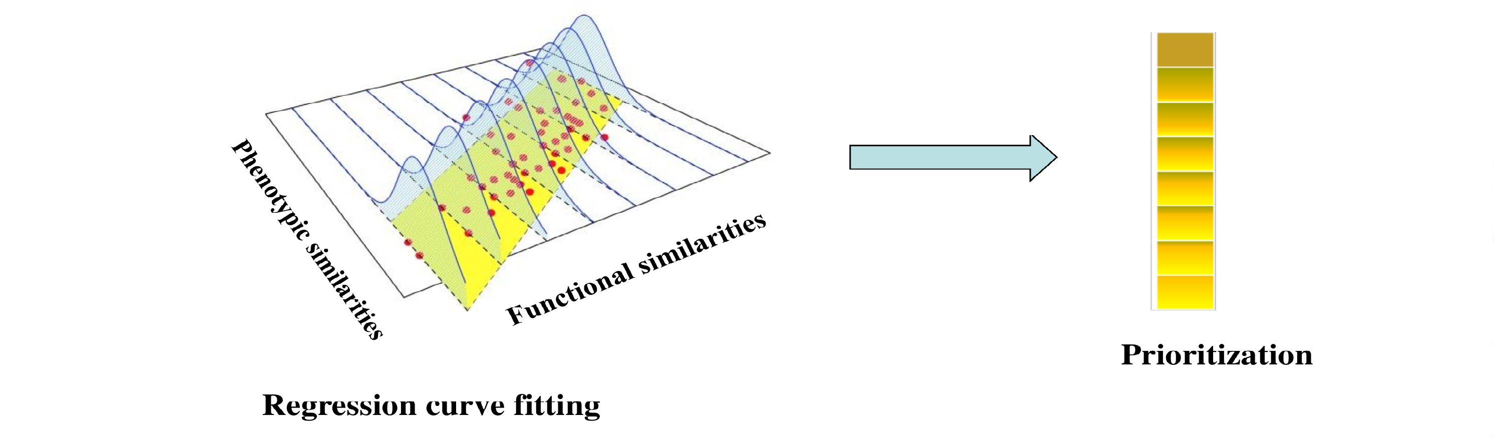
$$E(X\beta \mid y,\sigma_{\varepsilon}^2,\sigma_{\beta}^2) = XE(\beta \mid y, \sigma_{\varepsilon}^2,\sigma_{\beta}^2) \\ y_{pred} = E(X\beta \mid y,\sigma_{\varepsilon}^2,\sigma_{\beta}^2) = X\left[ X^T X + \tilde{\lambda} I\right]^{-1}X^T y$$